You can use a WINDOW statement in a transformation to compute values for each row based on values from a group of rows. For example, you could use WINDOW to rank purchases by size in each product category. (See the first example below.)

WINDOW statements give you a way to include windowing and aggregating functions in a script. Each windowing or aggregating function operates on a neighborhood of related rows, known as a window frame. Common examples of windowing functions are moving averages, cumulative sums, row numbering and ranking. (Examples follow.)

Supported Functions

A variety of aggregating functions are supported for use in WINDOW statements. See Aggregate Functions.

Reference

The syntax for a WINDOW statement is defined as follows:

WINDOW select_list BY partition_key [ORDER BY sort_expression [sort_expression …]]

Where:

• select_list is a list of comma-separated named expressions that may contain windowing functions or aggregating functions. A named expression requires you to specify an attribute (for example, rank() AS sales_rank). For each row in the table, these expressions are computed over the current window frame.
• partition_key is a list of variables that are used to divide the data into window frames, similar to the key in a GROUP BY statement. partition_key cannot be empty.
• Optional. ORDER BY can be used to create rolling window frames. The rolling window frame starts at the first row, and adds one row at a time to the computation until all rows have been evaluated. For example, it computes the cumulative sum for the top row, then the top two rows, then the top three rows, and so on, until the frame is complete. If you don't include the ORDER BY clause in the WINDOW statement, all rows in the window frame are included at once.

Tip: Most windowing functions, including rank() and row_number(), require adding an ORDER BY statement. Aggregating functions do not require an ORDER BY, but you may optionally include it.

Maintaining Row Order

Exporting the unified dataset after applying a WINDOW statement does not maintain row order. You can supply values for an attribute using the rank() or row_number() functions and then sort on these columns after exporting to reapply a row order.

Examples

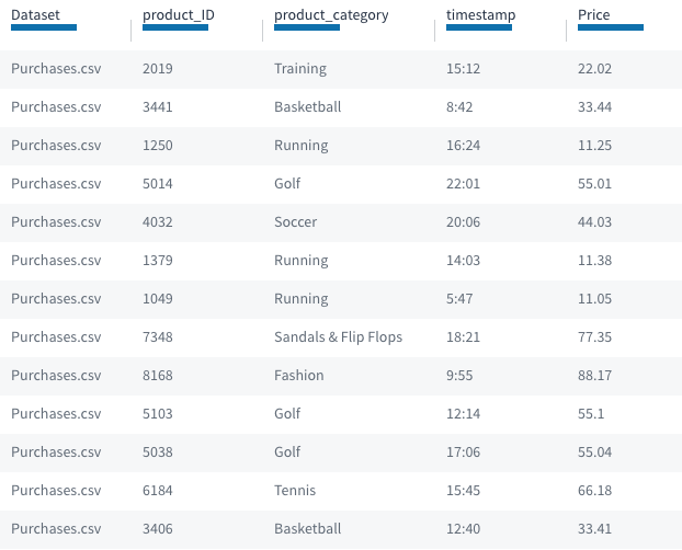
Suppose you have an input dataset of sales transactions data from an e-commerce site. It might look like the following:

rank()

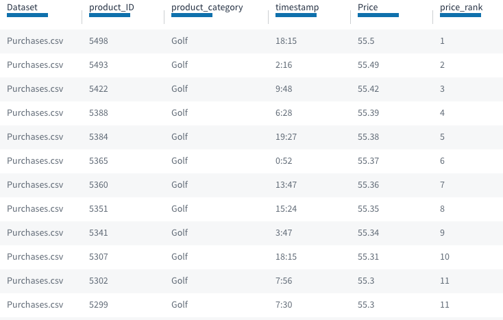
Now suppose that you’d like to rank the purchases by size in each product category (total sales per category) so that you can find the big purchases. You can use the following transformation:

WINDOW rank() AS price_rank BY product_category ORDER BY price DESC NULLS LAST;

This statement will partition the purchases by category, sort within each category by price, then compute the rank of each purchase. Here’s the result:

Choosing rank() vs. row_number()

When you use the rank() function, if two purchases have the same price they receive the same rank.

If you use the row_number() function instead of rank() then any tie values between purchases in a product category are arbitrarily ordered. Each time the WINDOW statement is run, the ordering between the tied purchases can change.

sum()

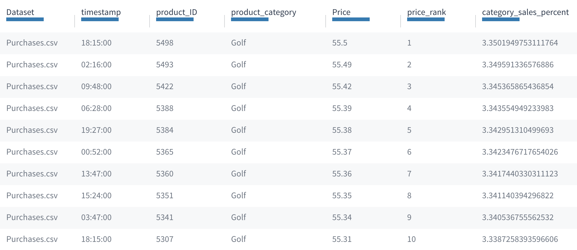
While ranking can be useful, suppose you want a more quantitative measure. Say you'd like to compare purchases based on what fraction of overall daily revenue they represent within their product category. You can use the sum() function to find the total within each category, and use it to compute the percentage each sale represents.

WINDOW Price, 100.0 * Price / sum(Price) AS category_sales_percent BY product_category;

For each row, this statement will fill the category_sales_percent column with that (row’s price) divided by (the total sales within the row’s category), times (100) to convert to a percent. Here’s the result:

The value in category_sales_percent is the same as if you'd used it in a GROUP BY transformation. Unlike a GROUP BY, however, here the output dataset has the same number of rows as the input, instead of only one row per group.

Now suppose you’re interested in daily trends. What time of day are customers spending the most? Maybe you want to see the distribution of sales by time within each product category.

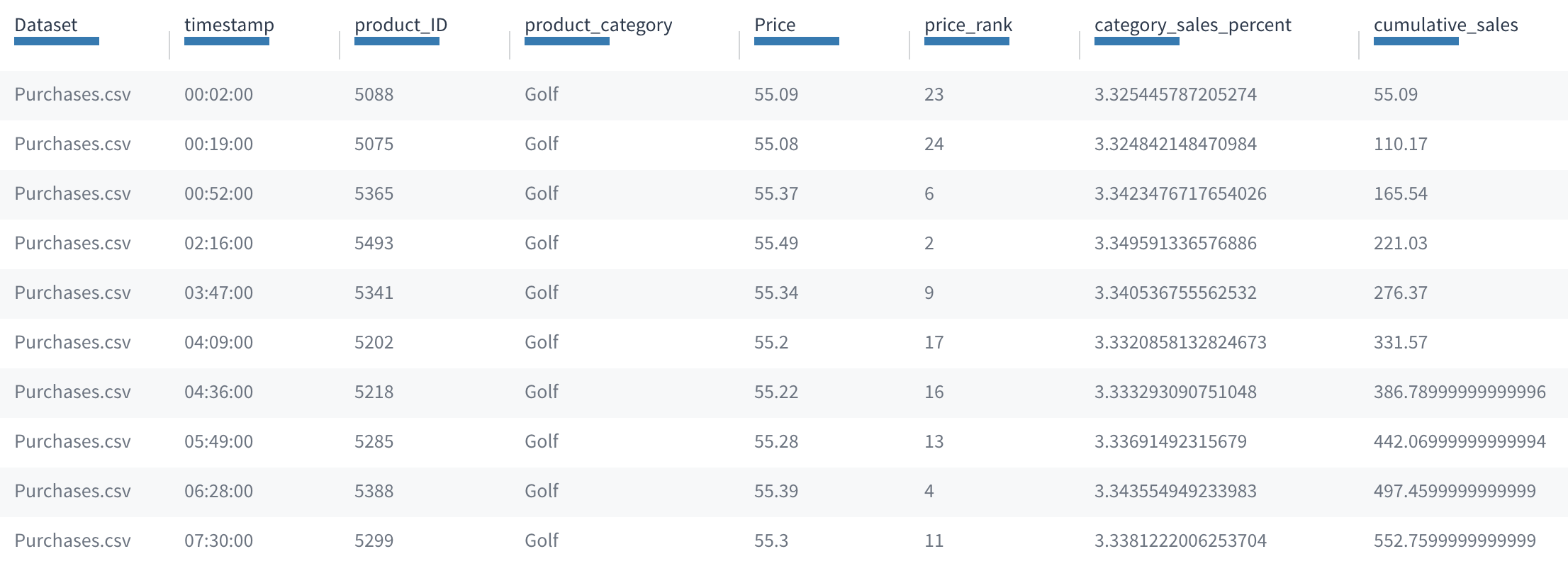
You can modify the last transformation by adding an ORDER BY clause to look for trends during the day:

WINDOW Price, sum(Price) AS cumulative_sales BY product_category ORDER BY timestamp;

For each purchase this script populates the cumulative_sales column with the total sales up to the current row’s time of day. In the table, you can see the cumulative_sales grow in each row:

Notice that with the ORDER BY clause the window frame is rolling. So rather than considering the whole partition, each row’s cumulative_sales sums only the rows preceding the current row’s time of day.

lag and lead

Instead of calculating a cumulative value, you can also specify your WINDOW statement to look at a row before or after the current row. This is useful when you want to calculate the change between two rows, for example.

You can write a lag() in the select_list expression to reference a row before, or a lead() to reference a row after. The format is lag(attribute, integer) or lead(attribute, integer). The integer indicates how many rows before, or after, the expression references. The integer must be positive.

Note: You must include an ORDER BY statement if you are using lag() or lead(). Be sure to consider the order you want, since this changes which row these functions reference.

For example, WINDOW Price, lead(Price,1) - Price AS Price_diff, BY product_category ORDER BY timestamp produces a table with rows ordered by the timestamp for each product_category, and the column Price_diff contains the difference between the two prices: the price of the current row minus the price of the row after. The Price_diff for the last row is null since there is no row after it.

Custom Window Frames

Overview

For each row, the frame of a WINDOW statement defines the set of records that are the inputs to the window expressions for that row. The frame defines a local context for each row: essentially, how many rows before or after, or before and after, the current row are included in the computation.

To give some examples, for a ranking window expression like row_number(), the frame is the current row and all the rows preceding it: row_number() returns the count of rows in the frame. For a 10-day moving average like avg(price), the window frame is the current row plus rows from the previous ten days.

A WINDOW statement can either use the default window frame, or else define a custom window frame explicitly.

Syntax

The syntax for a WINDOW statement with a custom window frame is as follows:

WINDOW select_list BY partition_key [ORDER BY sort_expression [sort_expression …]] frame_clause;

The frame_clause can be one of the following:

• ROWS frame_start
• RANGE frame_start
• ROWS BETWEEN frame_start AND frame_end
• RANGE BETWEEN frame_start AND frame_end

where frame_start and frame_end can be:

• UNBOUNDED PRECEDING
• value PRECEDING
• CURRENT ROW
• value FOLLOWING
• UNBOUNDED FOLLOWING

If you omit frame_end it defaults to CURRENT ROW.

There are a few rules for using frame_start and frame_end:

• frame_start cannot be UNBOUNDED FOLLOWING
• frame_end cannot be UNBOUNDED PRECEDING
• The frame_end choice cannot appear earlier in the above list than the frame_start choice. For example, RANGE BETWEEN CURRENT ROW AND value PRECEDING is not allowed
• value must be a non-negative integer

ROWS vs RANGE

The window frame defines an ordered set of rows before and after, or before and after, the current row. UNBOUNDED PRECEDING and UNBOUNDED FOLLOWING denote all rows in the current partition before and after the current row, respectively. The meaning of CURRENT ROW depends on whether ROWS or RANGE is specified. In ROWS mode, CURRENT ROW means the current row, only. In RANGE mode, it means all rows that have the same value in the ORDER BY expression as the CURRENT ROW.

The meaning of value PRECEDING and value FOLLOWING also depends on whether ROWS or RANGE is specified. In ROWS mode, value indicates the number of rows before or after the current row, respectively, to include. In RANGE mode, value indicates the range to include based on values in the ORDER BY expression. For example, for the WINDOW statement:

WINDOW sum(Price) AS new_Price BY product_category ORDER BY timestamp RANGE 1 PRECEDING;

Then new_Price for each row sums up the current row’s price with that of all rows on the same timestamp or from one timestamp before in that product category.

RANGE frames require an ORDER BY clause, and the ORDER BY clause must have exactly one sort expression of numeric data type. Equal values in the ORDER BY expression are all treated the same. That means in RANGE, CURRENT ROW means the current row plus all rows with an identical value in the ORDER BY expression.

Note: Windowing functions, including the offset window functions lag() and lead(), define their own implicit window frames and are therefore incompatible with custom window frames. These functions can only be used with the default window frame.

Default Window Frames

The default window frame depends on the expressions in the expression list, and on whether there’s an ORDER BY clause or not.

If there is no ORDER BY clause, then the default window frame is:

ROWS BETWEEN UNBOUNDED PRECEDING AND UNBOUNDED FOLLOWING

That is, it’s the whole partition. The result is that every row in a partition computes the same value for each window expression. This is equivalent to a GROUP BY statement that does not merge together the rows in each partition.

ORDER BY without Offset Window Functions

When there is an ORDER BY statement and the window expressions do not include any window functions then the default window frame is:

RANGE BETWEEN UNBOUNDED PRECEDING AND CURRENT ROW

That is, all the rows in the partition before the current one, plus any rows with the same value as the current row in the sort expression.

ORDER BY with Offset Window Functions

Offset window functions define their own window frames implicitly to match the function semantics. For example, lag(Price, 10) has the implicit window frame:

ROWS BETWEEN 10 PRECEDING AND 10 PRECEDING

That is, the offset functions set the frame to match the row they select exactly. You can define multiple offset window functions in the same expression or in the same WINDOW statement. Tamr Core sorts out how to combine all of the window frames appropriately. (That is, one frame is applied to each offset window function.)